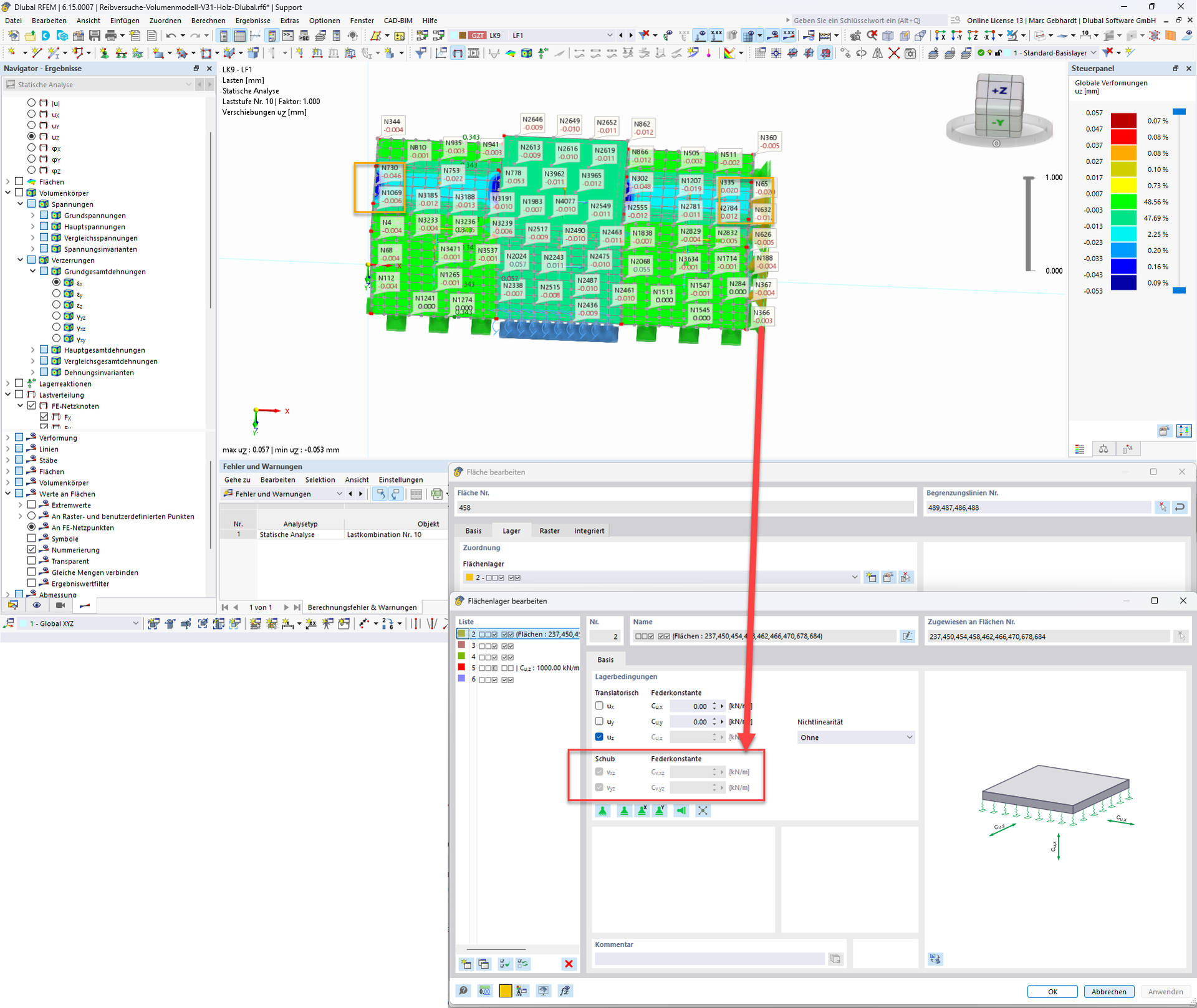
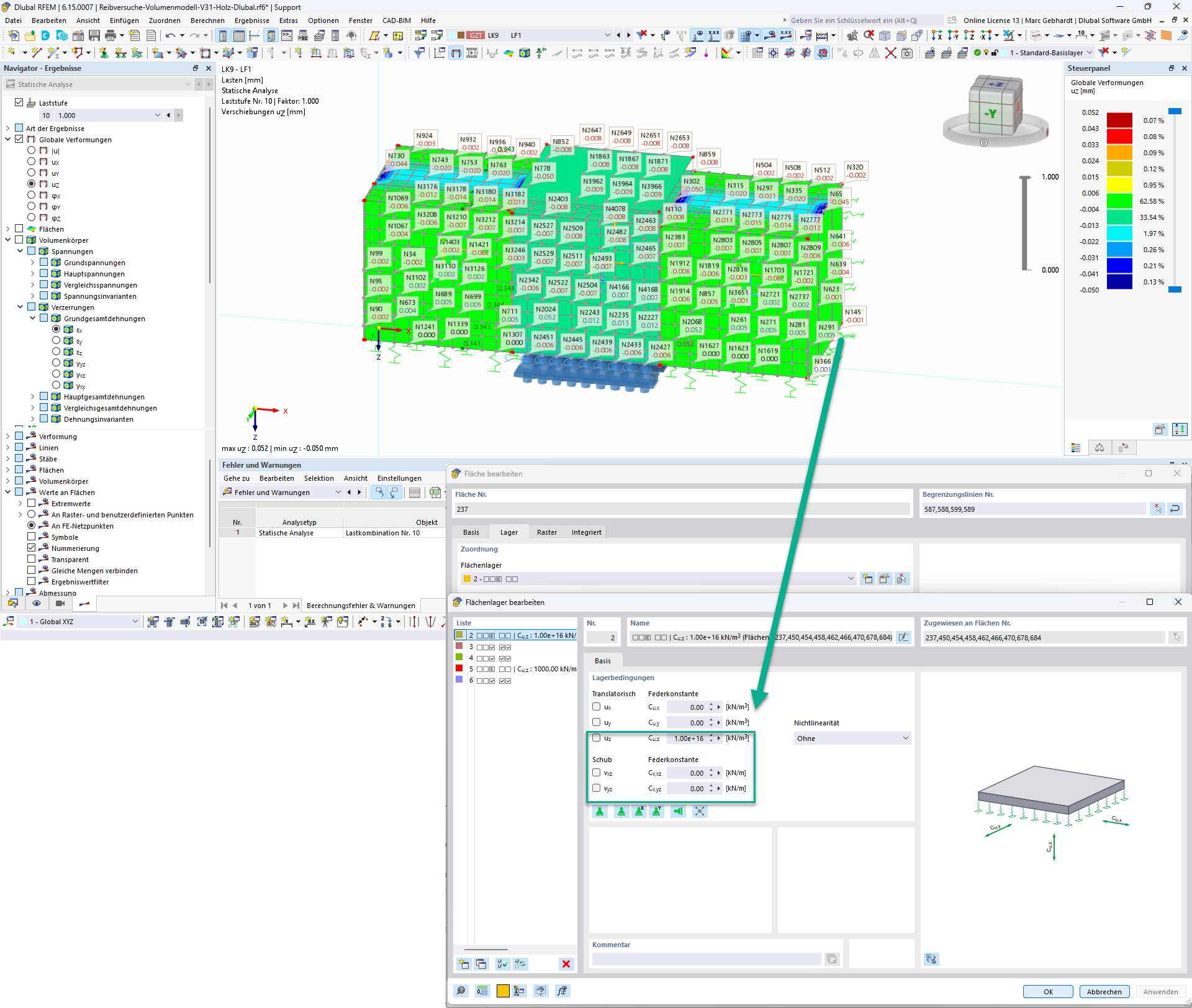
Modeling of friction – contact volume

[AlexITI]

Dear Dlubal community,

I have a question regarding the modeling of friction in volumetric models.

In my opinion, friction works well in surface elements in RFEM 6. As I understand it, exceeding the static friction can be well represented by means of virtual nodes and visible node displacements in the friction surface.

I think friction works differently in volumetric elements. Since friction between two parallel surfaces lying in one plane cannot be generated via surface contact, I have resorted to contact volumes. In contact volumes, the connection of the nodes in the shear surface is established via the contact volume. When the static friction is exceeded, there is a displacement of the nodes, which is represented by a distortion of the contact volume.

Have I basically understood the integration of friction in RFEM 6 correctly?

In this context, I have a question regarding the correct input of the values for the contact volume. For example, I can define a static friction coefficient, but I must also assign the material a stiffness using the modulus of elasticity. On one hand, how does the modulus of elasticity affect the transmission of local stress peaks between volumetric elements (is a lower modulus of elasticity better so that local peaks are not absorbed), and on the other hand, how does it affect the transferable shear forces in the shear joint (is a higher modulus of elasticity better so that distortions are influenced only by the friction coefficient and not by the modulus of elasticity)?

Can someone help me regarding this?

Best regards
Alexander Gerger

[marc.gebhardt]

Hello Alexander,

First, I would like to address the different types of contact modeling for the connection of surfaces: Here, besides the rigid connection, surface releases, surface contacts, and contact volumes are available. These differ in their approach and thus also in their effects on the structural system.

• Surface releases release the degrees of freedom under certain conditions where these share a location (overlap). We are currently working on the implementation of nonlinearities such as the friction contact described here.
• Surface contacts establish a connection of the degrees of freedom between surfaces with a gap.
• Contact volumes function geometrically like surface contacts. However, the stiffness of the volume from geometry and material is incorporated here.

Since friction between volumetric bodies should be assumed to occur at the contact surfaces, the influence of the contact should be minimized. This can be achieved by a very small gap and, in the case of a contact volume, with high material stiffness.

The typical use of contact volumes is, especially historically, the connection of two surfaces modeled at their centroids. The recommendation here would be to choose the material with the lower stiffness of the connected elements. Another use case is the connection using an adhesive/polymer, for example for volumetric bodies, where the material properties of the bonding material should be applied.

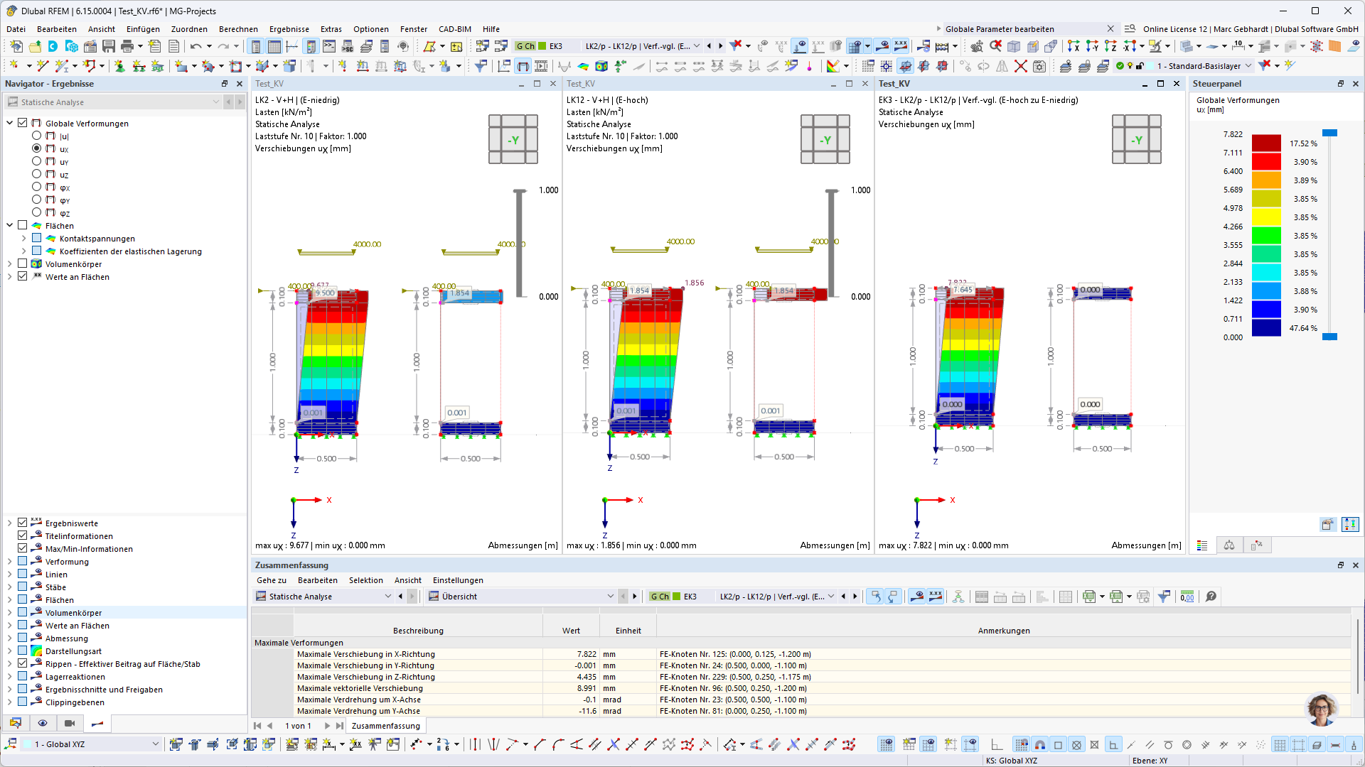
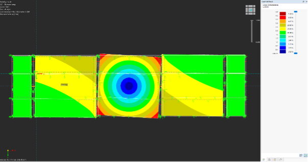
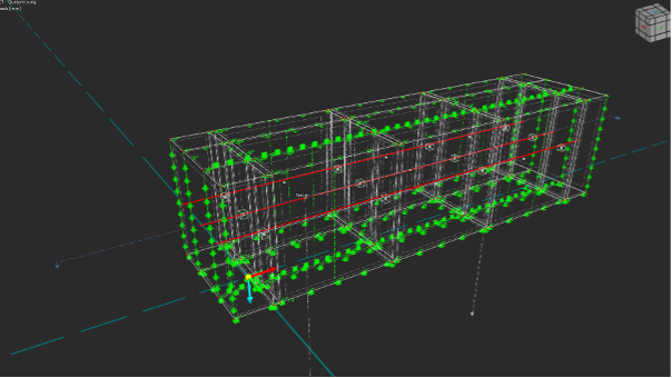
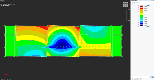
To test the influence of the stiffness of the contact volume on the friction connection, I have prepared and attached a small model. The same condition is modeled in two ways here: on the left by means of a contact volume and on the right by means of a surface contact. Additionally, the material of the contact volume was exchanged via the design situation. The deformation in the horizontal direction is shown in the following image. From left to right, the results with a low and a high modulus of elasticity of the contact volume, as well as their difference determined by result combination, are shown. As this shows, the influence is not negligible. In this example, the pure friction displacement is 1.85 mm, whereas the deformation due to the stiffness of the contact volume is 7.65 mm.

Test_KV-nr.rf6 (1.3 MB)

Best regards
Marc

[AlexITI]

Hello Marc,

Thank you very much for your response! This clarifies the influence of the stiffness of the contact volume. I have already tested the different options for modeling contact & friction in RFEM 6, but have not yet found a completely satisfactory solution.

• Surface releases (do not yet have friction)

• Surface contacts have a problem with the contact condition in my specific case, as the solids begin to slide into each other even at low load steps (0.14-0.16). Regardless of the number of load steps (tested up to 500). I have attached the model.

• Contact volumes allow the correct representation of contact through "prestressing" (no sliding of the solids into each other).

However, when transferring friction I encounter a problem. When I apply shear forces as a "displacement-controlled test" through imposed nodal displacements, I get results, but the static friction range (before sliding) cannot be represented correctly because I am forcing a displacement. I have attached the model.

In the case of a "force-controlled test," I get no results because my system becomes unstable. I am still troubleshooting this.

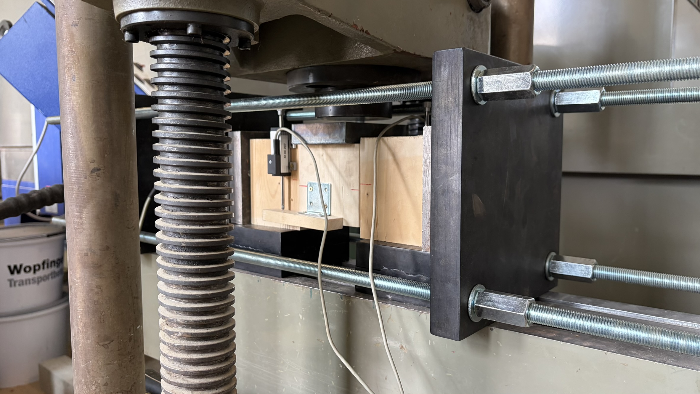
What would be your recommendation for this specific case? I've also attached a photo of the test setup again.

Best regards
Alexander

Reibversuche-Dlubal-Flächenkontakt.rf6bak.zip (1.4 MB)
Reibversuche-Dlubal-Kontaktvolumen-verschiebungsgesteuert.rf6.zip (2.5 MB)

[marc.gebhardt]

Hello Alexander,

Thank you very much for your feedback. A truly very interesting project! If this is part of your thesis, we would be very happy to receive the submission from you after completion!

Now to your model and the associated question:
First, however, we should explain the implemented features so that everyone can follow this thread afterwards. In my opinion, the idealized Coulomb friction is implemented in RFEM. This means that static and kinetic friction are the same. Before sliding, the shear force increases (rigid or elastic) until μ⋅σ, or τ_max, is reached.
During sliding, the shear force then remains constant at μ⋅σ, or τ_max. However, this also means that without stops or numerical springs as supports, a rigid-body displacement may occur. In my opinion, this is the instability that is being reported to you. Generally, neglecting higher static friction is on the safe side, and the verification only considers the kinetic friction level. However, since an experiment is to be recalculated here, the simulation should be as realistic as possible. If I interpret this correctly, you have defined a nonlinear line support at the bottom using a diagram for the additional representation of static friction — Chapeau, that takes some ingenuity!!!

The problem of mutual displacement under load normal to the contact (preloading) seems to me to be an error and is related to the analysis according to third-order theory. I have forwarded this for review to our development department.

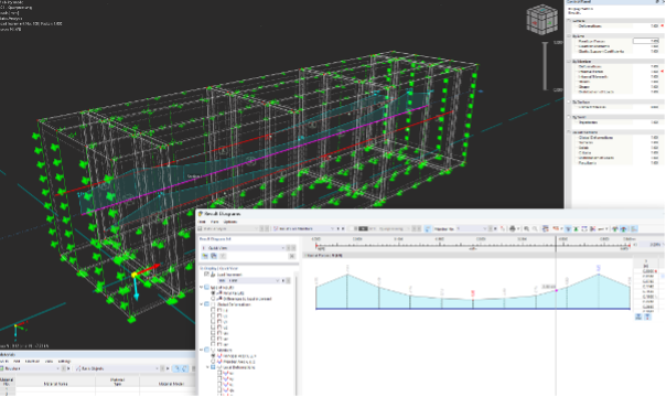
For evaluation, I can also recommend the calculation diagrams and our API. Possibly, our digital twin could also be helpful for matching the measured values. Furthermore, I have attached a model with a displacement-free support as inspiration.

Reibversuche-Volumenmodell-V11-3037-Flächenkontakt-mg-nr.rf6 (1.8 MB)

Best regards and continued success
Marc

[AlexITI]

Hallo Marc,

vielen Dank für deine Rückmeldung. Guter Hinweis – ich werde künftig bei Arbeiten an unserem Forschungsbereich anregen, Arbeiten bei euch einzureichen

Vielen Dank für deine Erläuterungen! Die Berechnungsdiagramme sind eine wirklich gute Funktion von euch! Auch dein Modell ist eine super Inspiration.

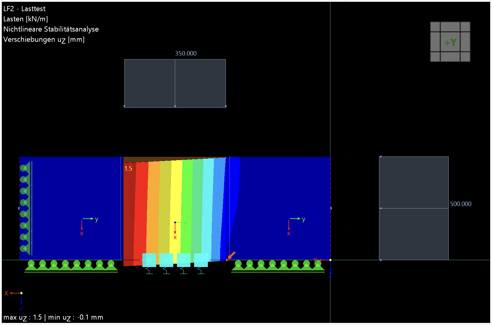
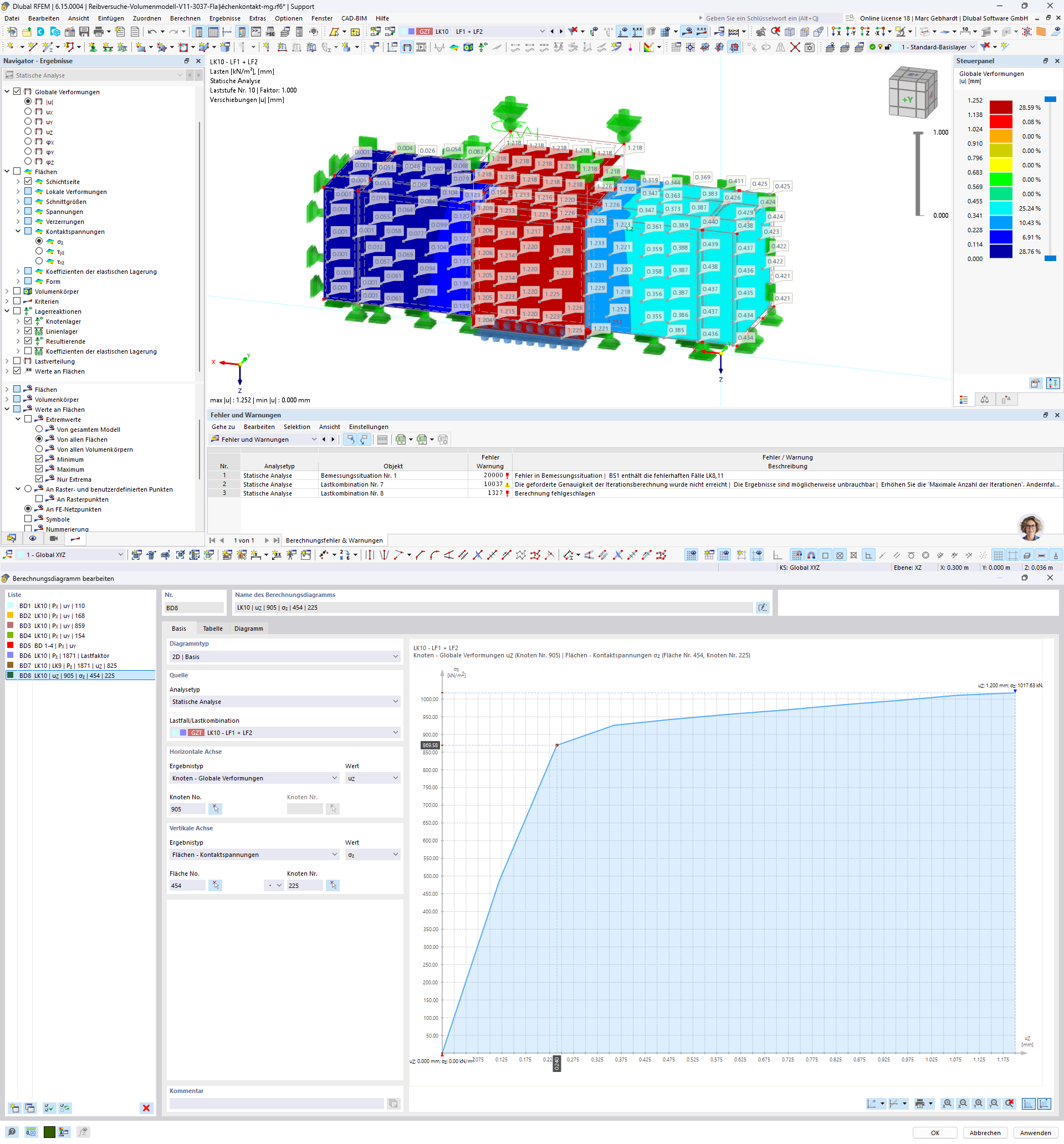
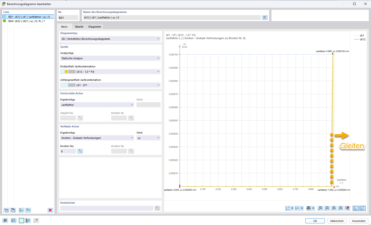
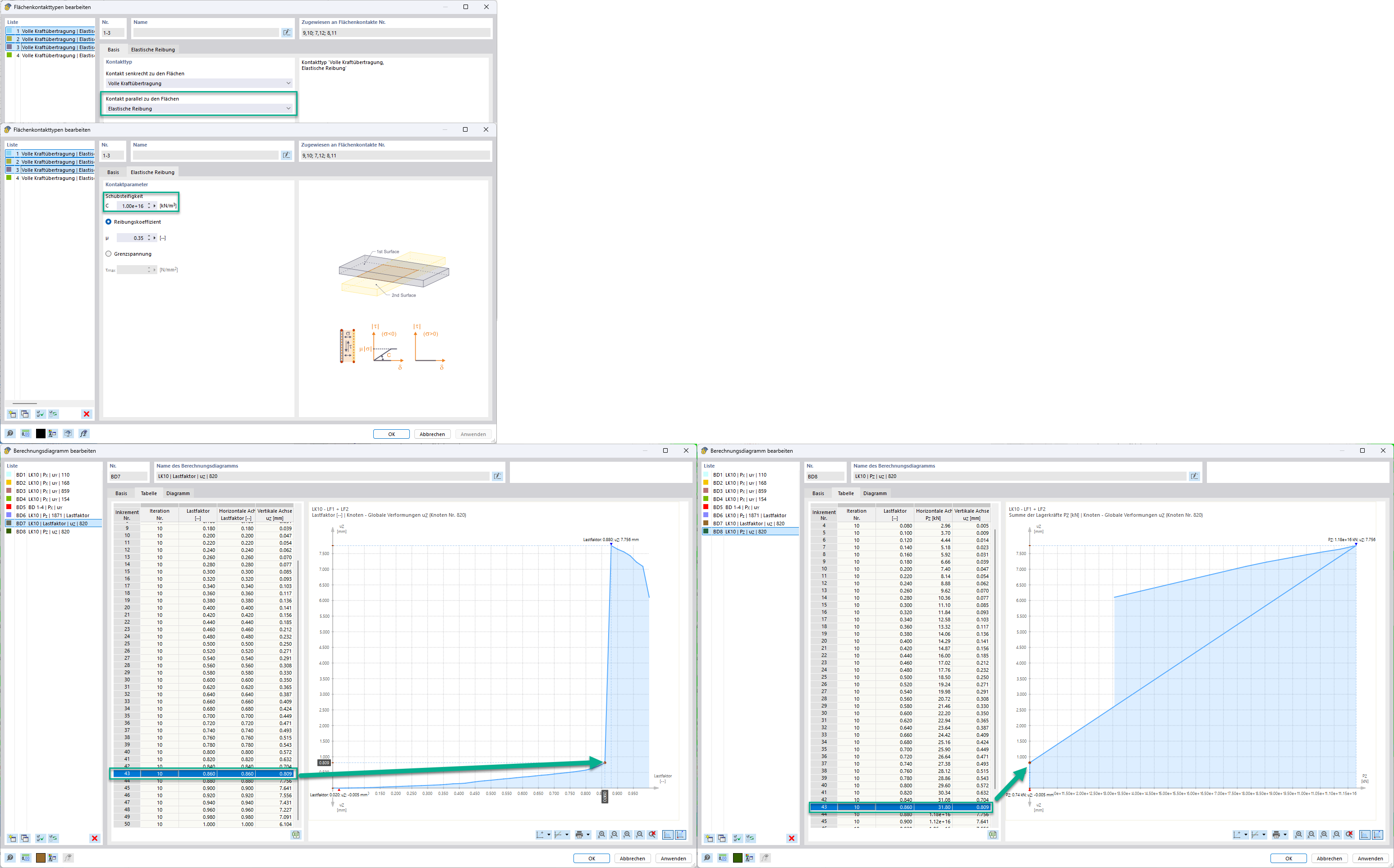
Die genaue Implementierung der Coulomb-Reibung verstehe ich noch nicht ganz – dazu gestatte mir bitte noch eine Nachfrage. Ich habe eine Vorspannung von 50kN. Bei einem Reibbeiwert von 0.35 in den Flächenkontakten müsste bei 2 Reibflächen eine Scherkraft von 0,35*50*2=35kN übertragen werden können, BEVOR das System zu gleiten beginnt. Etwaige Verformungen in diesem Bereich resultieren aus Deformation der Körper selbst ohne Starrkörperverschiebungen. Diese sollten ca. 1,2mm betragen. Bei einer Aufbringung der Scherkraft von 35kN (kraftgesteuert) mittels Laststufen erhalte ich jedoch bereits zu Beginn bei Laststufe 0.28 eine (Starrkörper)verschiebung von 1,2mm (siehe Berechnungsdiagramm anbei). Das Diagramm zeigt, dass es keinen Haftreibungsbereich gibt, sondern sofort ab Belastungsbeginn ein Gleiten eintritt. Das sollte doch eigentlich nicht sein – oder verstehe ich etwas falsch? Der starke Anstieg ab 5mm resultiert aus meinen Einstellungen zur Bettung in z-Richtung.
Reibversuche-Volumenmodell-V11-3037-FK-kraftgesteuert-mg-nr-NoResults.rf6.zip (1,5 MB)

Danke für die Weiterleitung des Problems beim Flächenkontakt. Könntet ihr mich informieren, wenn es dazu Lösungen gibt?

Wir haben in der Zwischenzeit mit den Kontaktvolumen weiter getestet und folgendes Problem festgestellt: bei einem völlig symmetrischen System und symmetrischer Belastung kommt es zu einer Rotationsbewegung – woher? Die Körper sind nicht starr sondern nachgiebig mittels Flächenbettung gegen Verdrehung um die globale Z-Achse gelagert. Die beiden Lasteinleitungsplatten sind für eine flächentreue Lasteinleitung sogar durch eine x-parallele-Wegführung gelagert, die jedenfalls an den Enden eine Rotation ausschließt.
Reibversuche-Volumenmodell-V10-2A_Quad_5mm_Elastic._Delete3_LoadMovement_NoResults.rf6.zip (2,0 MB)

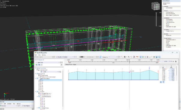
Die Auswertung mittels Ergebnislinie zeigt einen „seltsamen“ nicht konstanten Normalkraftverlauf.

Selbst nach Variation der Lagerung zu einem immer steifer gehaltenen System (feste Y-Z-Haltung der Lasteinleitungsflächen und Y-Linien-Haltung aller Solid-Elemente oben und unten) verdreht sich das System immer noch.
Reibversuche-Volumenmodell-V10-2A_Quad_5mm_Elastic._Delete3_LoadMovement3_NoResult.rf6.zip (2,1 MB)

Ich vermute auch hier ein Problem mit der Berechnung nach Theorie III.Ordnung?

Vielen Dank für deine Hilfe und

LG
Alexander

[marc.gebhardt]

Hallo Alexander,

@AlexITI

vielen Dank für deine Rückmeldung. Guter Hinweis – ich werde künftig bei Arbeiten an unserem Forschungsbereich anregen, Arbeiten bei euch einzureichen

Das wäre super, danke!!!

Aktuell erfolgt die Benachrichtigung über Extranet. Im Bereich Entwicklung ist eine Übersicht über geplante Features sowie eine Auflistung der gemeldeten und behobenen Fehler auffindbar. Bezüglich einer direkten Benachrichtigung habe ich dich in den zugehörigen Kundenwunsch hinzugefügt.

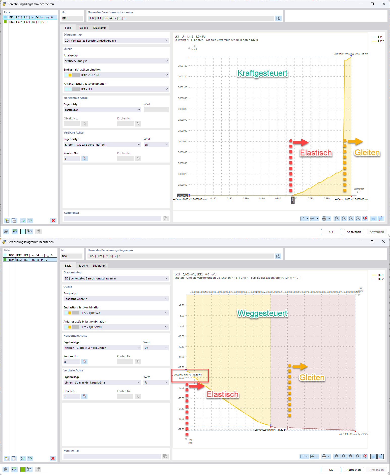
Das ist tatsächlich nur schwer erklärbar. Ich habe für den schnellen Test hierfür ein Trivialmodell angelegt. Dieses besteht aus drei annähernd starren Flächen, die mittels Flächenkontakten und starrer Reibung verbunden sind. Die äußeren Flächen sind, soweit vereinfacht möglich, zwängungsfrei gelagert und die mittlere wird horizontal, kraft- oder weggesteuert inkrementell belastet. Für die kraftgesteuerte Analyse ist des Weiteren ein Anschlag ab 0,0001 mm Verformung hinzugefügt. Nachfolgende Bilder visualisieren meine Beobachtungen. Den größten Unterschied zeigt hier die Steifigkeit der verwendeten Flächen.
Trivial_test_Reibkontakt_zf_FK.rf6 (1,2 MB)

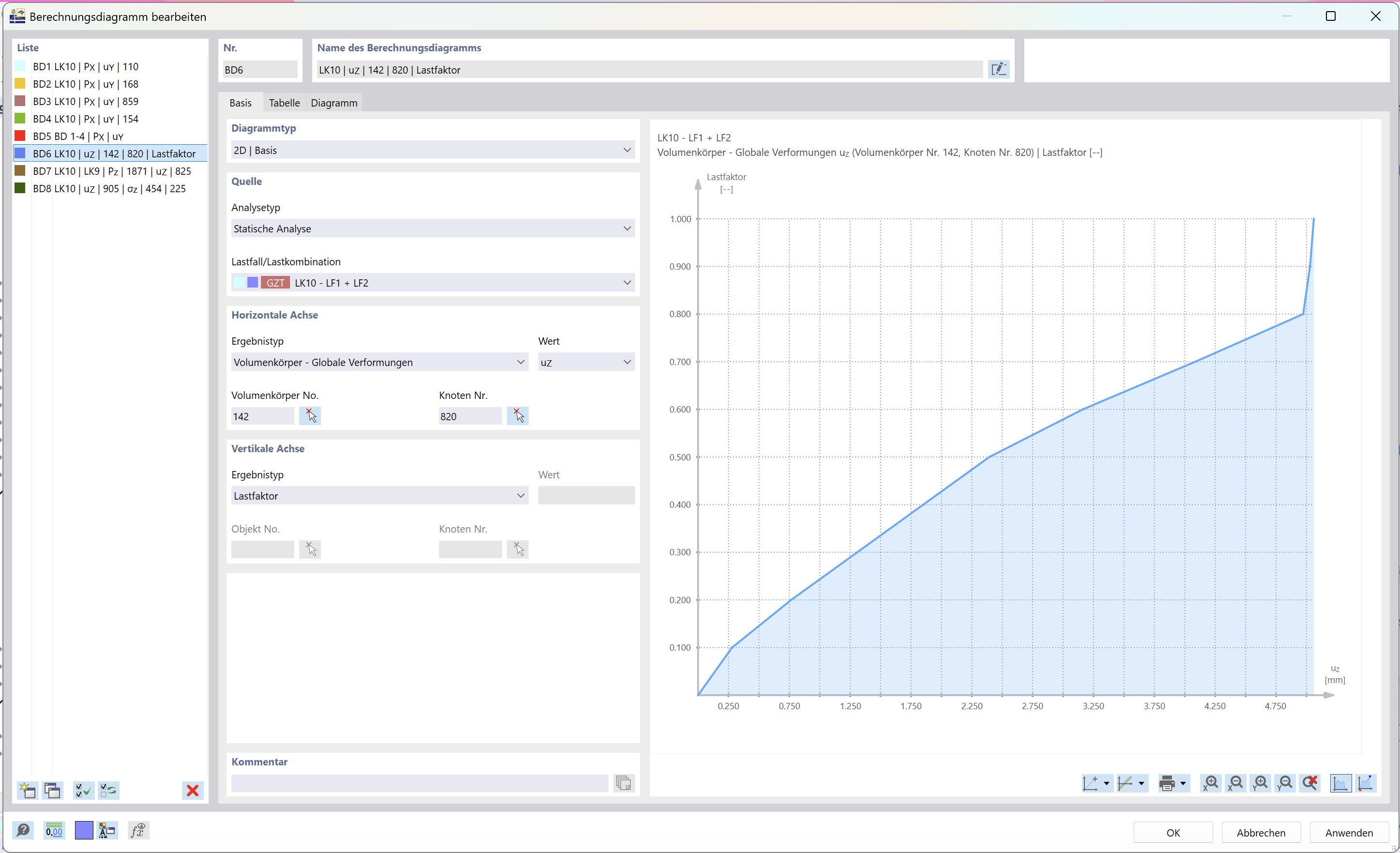
Bei einem E-Modul von 1e9 MPa beginnt bereits ab einem Lastfaktor von 0,63 (F~22 kN) eine elastische Verformung. Gleiten tritt ab einem Lastfaktor von 0,95 (F~33 kN) auf. Noch interessanter verhält sich dies bei der darunter gezeigten weggesteuerten Simulation. Hier beginnt das Diagramm mit dem elastischen Verhalten unter einer resultierenden Anfangskraft von 18,4 kN bis sich bei rund 33 kN Gleiten einstellt.

Wenn wir den Elastizitätsmodul auf 1e13 MPa erhöhen, kann man den Unterschied sehr gut in der kraftgesteuerten Analyse sehen. Hier gibt es keinen ausgezeichneten elastischen Bereich und Gleiten tritt ab einem Lastfaktor von 0.99 (F~34.7 kN) ein.

Die Berechnung nach Theorie III. Ordnung würde ich in diesem Fall nicht empfehlen, vor allem im Hinblick auf den gemeldeten Fehler, jedoch auch im Allgemeinen, da hier, meiner Auffassung nach, insbesondere der Bereich vorm Gleiten untersucht werden soll.

Beste Grüße und frohes Forschen
Marc

[AlexITI]

Hello Marc,

Thank you very much for your test. This confirms the fundamental possibility of modeling in RFEM – that is the most important information for me.
As soon as we have completed our project, we will gladly submit the FE models.

Best regards,
Alexander

[AlexITI]

Hello Marc,

Thanks again for your test. This one involved comparatively high material stiffnesses.
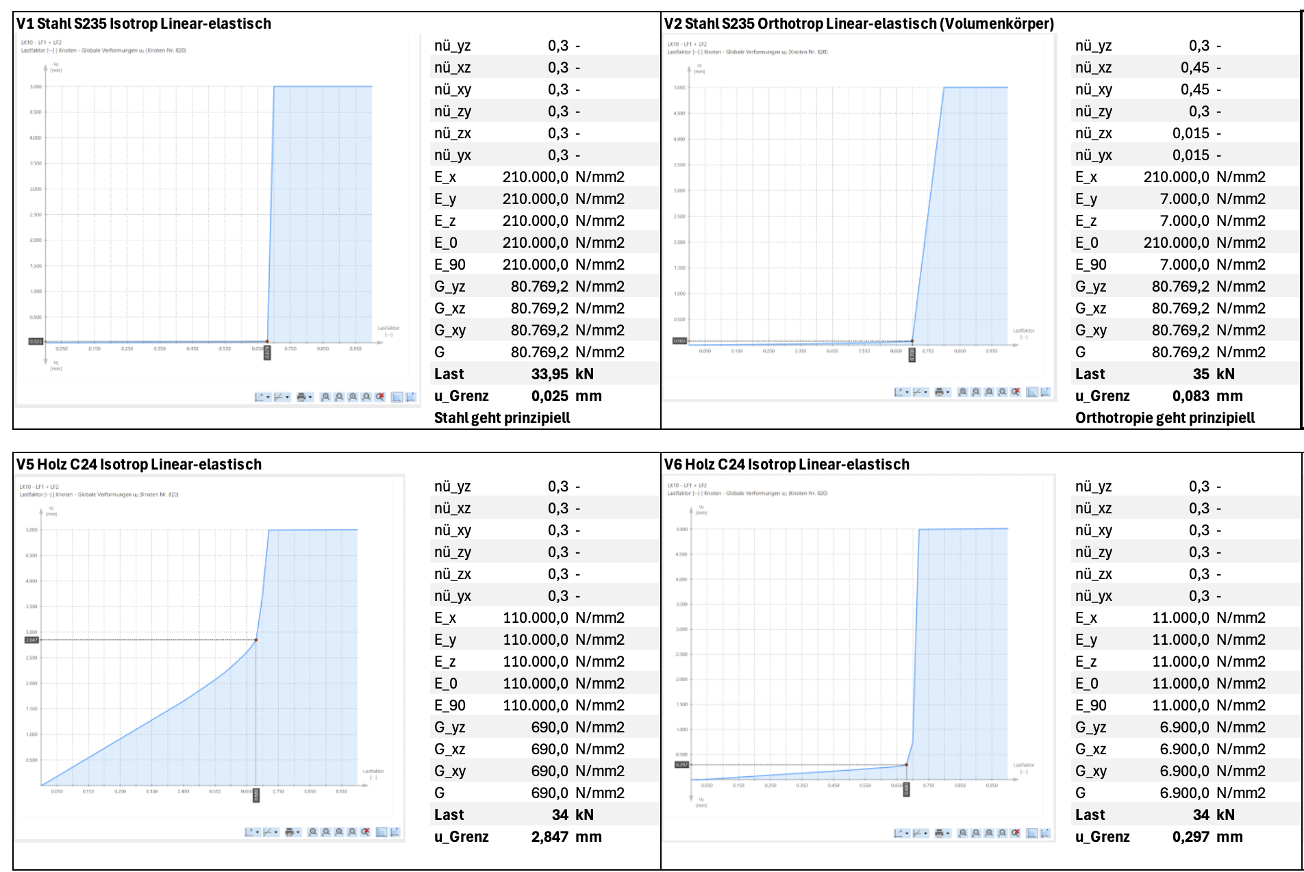
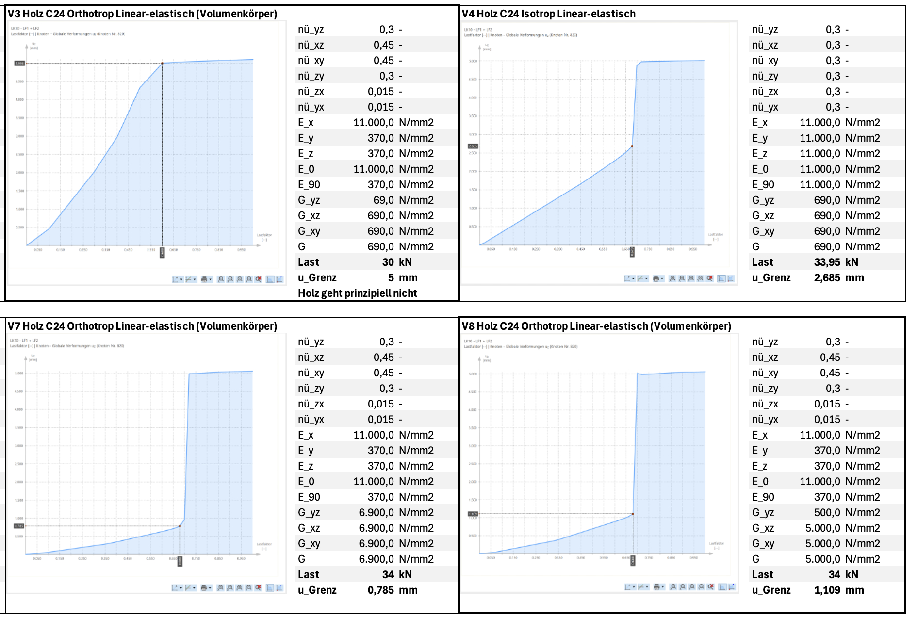
I have now done a small parameter variation to see where the problem lies with wood (BSP). Attached are the calculation diagrams.

V1 steel, isotropic, works well.
V3 wood, orthotropic, produces too large deformations before the transition from static to kinetic friction. In our tests, we observed a deformation of 1.2mm at about 35kN.
In my opinion, the decisive parameters are the shear moduli.

Since this is an analysis of the stresses for models to predict a rolling shear failure, simply increasing the shear moduli is not effective.

Is there a solution for this?

Best regards
Alexander Gerger

[marc.gebhardt]

Hello Alexander,

Thank you very much for sharing your results! Unfortunately, I still lack some understanding here. Therefore, please answer the following questions for me:

1. Which model does the parameter study refer to?
2. Was a surface contact with minimal clearance applied here, as recommended?
3. If the boundary displacement was measured as 1.2 mm at 35 kN, then the V8 variant is already quite close to the measured results. Or is there a flaw in my thinking here?

Correct, I would interpret it the same way. For the investigation of rolling shear failure, realistic shear moduli should be applied.

Best regards
Marc

[AlexITI]

Hello Marc,

Re 1.) Attached I’m sending you the model
Reibversuche-Volumenmodell-V20-Holz-Dlubal.rf6 (1.9 MB)

Re 2.) Yes, instead of contact volumes, surface contacts with minimal spacing were used. This seems to be the better option. Friction of stiff materials (e.g. steel) seems to be representable very well this way

Re 3.) That is correct. In variant V8 I deliberately experimented with which parameters need to be changed in order to match the measurement results. The shear moduli were increased by about a factor of 10 (69 -> 500, 690 -> 5000 N/mm²). So it is a dummy material.

The correct materials are only considered in two variants: steel (V1) and wood (V3). All other variants were only used to determine which material parameters are responsible. With correct material values for orthotropic wood and the modeling as a CLT element, much larger deformations occur than observed in the tests. In V3 no transition from static to kinetic friction can be observed within 5mm (tests 1, 2 mm). By varying the material parameters, it seems that the comparatively small shear moduli of wood have the greatest effect on these (too large) deformations.

Best regards
Alexander

[marc.gebhardt]

Hello Alexander,

First of all: Thank you for sending the file!

Unfortunately, I suspect that we are dealing with a general fitting problem here. When adjusting a simulation to an experiment, it is important to either eliminate or represent the possible influences. Furthermore, enough measurement data must be available to perform a reliable fitting.

In your case, I would assume that displacement and force were measured over time. In short, this only reflects the global system response. This can, of course, arise from different systems. From my point of view, uncertainties arise on the one hand from the static and kinetic friction approach and on the other hand from the material parameters.

• Were the material parameters determined in individual tests? Or were local deformations or strain fields measured?
• Was the influence of a faulty independent measurement basis considered?
• Were tests performed in which the connection of the elements along the fiber direction was examined individually? Possibly, different friction coefficients result here depending on the connected elements.
• How was the prestressing applied and was it documented throughout the test?
• Was a difference between static and kinetic friction measurable? Was the progression at least partially linearizable?

I have simplified your model again to reduce influences. Here, I assume that the load introduction plates are infinitely stiff and have no relevant friction. This reduces the friction contacts to the areas to be examined.
Reibversuche-Volumenmodell-V20-Holz-Dlubal-MGadj-nr.rf6 (1.8 MB)

In both this adapted and your original model, I was able to observe significant deformation of the volumes in the pre-critical region. This particularly affects the inner layers of the supported test specimens. Did you take this into account in your evaluation? (Especially in this point, the as realistic as possible approach of the material parameters would be crucial. For example, you equated Ey and Ez as well as Gxz and Gxy.) The elastic deformation of your overall system can hardly be neglected here. Simplified, your test setup results in bending of the middle body and shear distortion of the outer parts, accompanied by deformation of the contact surfaces.

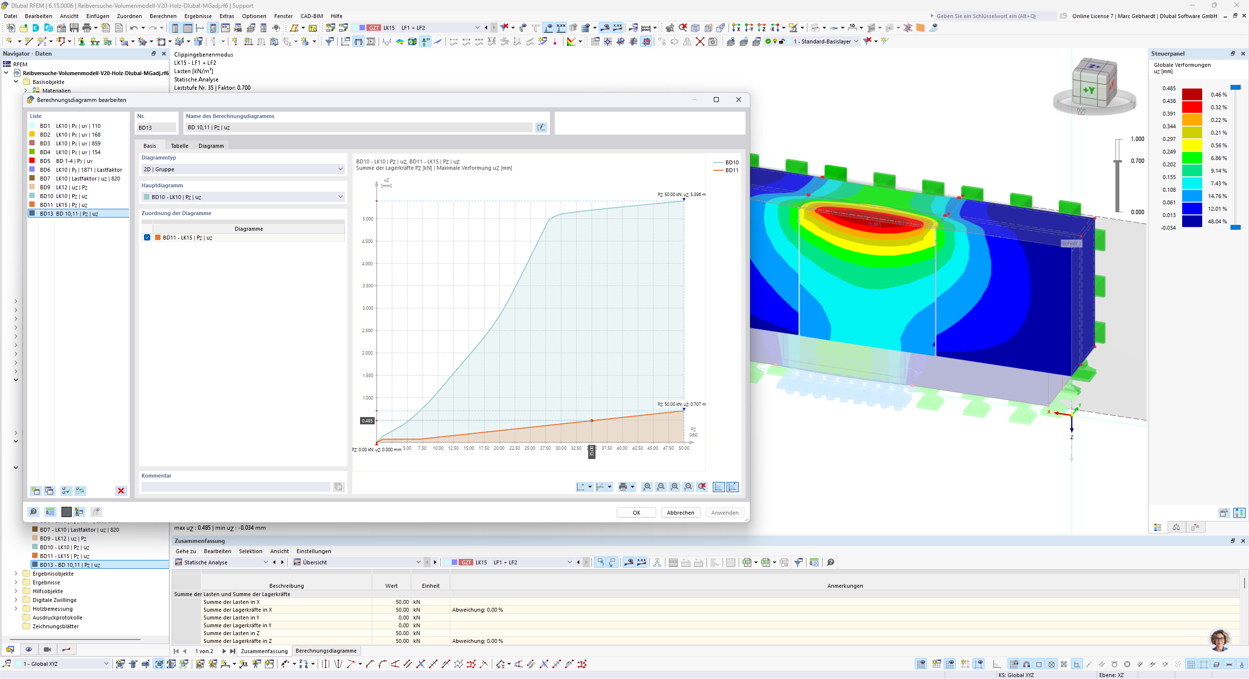
At 35 kN, in the attached example and neglecting contact nonlinearity, 0.485 mm of deformation is attributed to the purely linear-elastic portion:

Possibly, a parameter study could also be carried out here using the API. It would be conceivable to set different friction coefficients between the cross-sectional parts and vary the material parameters within narrow limits. This technical article describes the execution of parameter studies based on global parameters using the API. In the end, you could at least identify parameter combinations for a match or sensitivities.

However, the fitting becomes problematic if behavior not corresponding to our friction model, e.g. nonlinear progression, is underlying.

I hope I could help you! In any case, model training or validation and inverse analysis is always an incredibly exciting topic!

Best regards
Marc

[AlexITI]

Hallo Marc,

vielen Dank für deine Antwort!
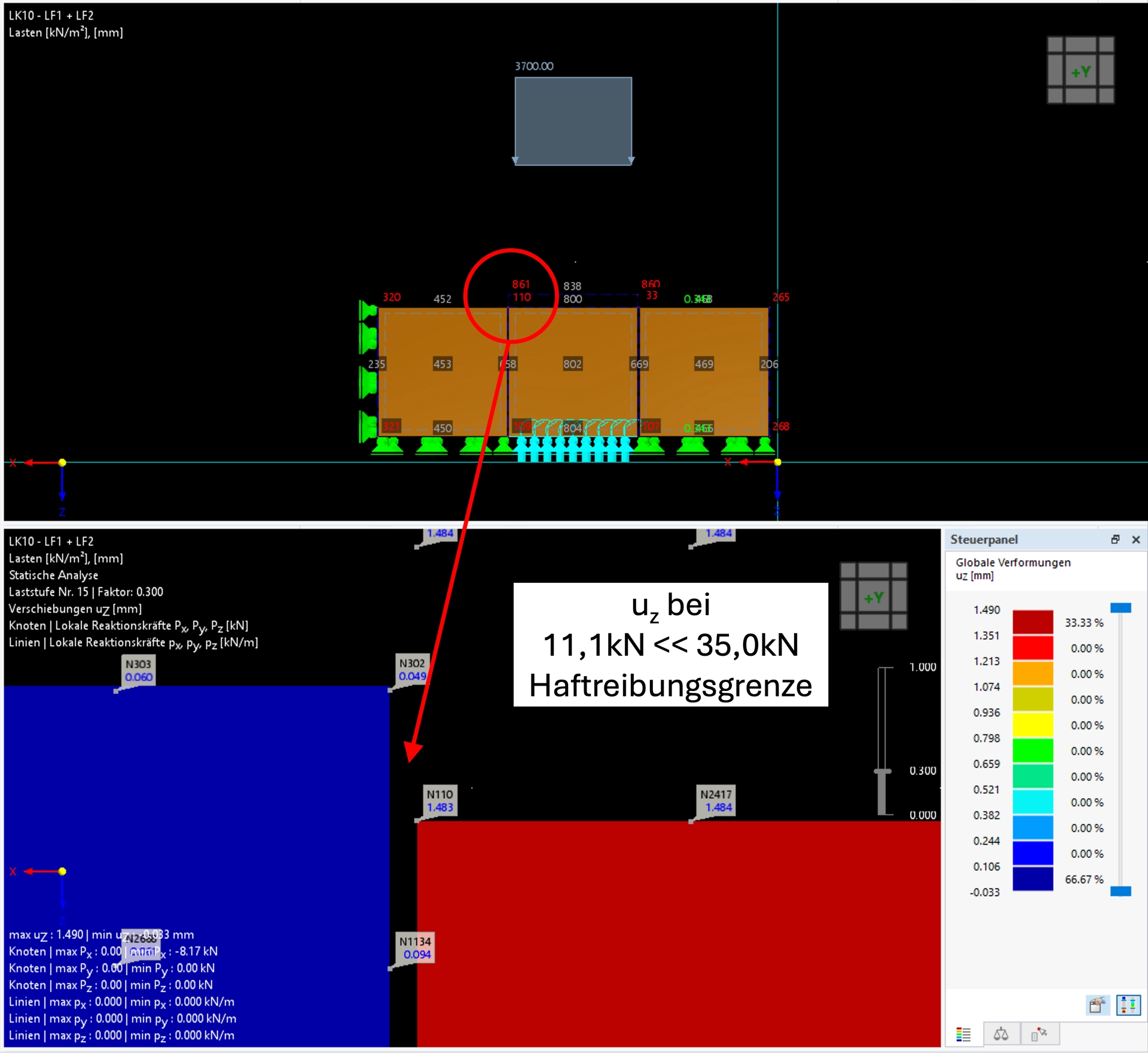
Ich stimme dir zu, dass das Gesamtsystem im Haftbereich relevante Verformungen (Deformationen) aufweist – diese haben wir mit ca. 1,2mm auch in den Versuchen gemessen. E- und G-Modul sind entsprechend Herstellerdaten angewendet worden. Ich stimme dir ebenfalls zu, dass der mittlere Versuchskörper einer Biegebeanspruchung ausgesetzt wird, währen die Decklamellen erheblichen Schubverzerrungen ausgesetzt sind. Jedoch zeigt das RFEM-Modell nicht dieses Verhalten. Es kommt bereits ab niedriger Belastung zu dominanten Gleiten anstelle von signifikanten materiellen Deformationen in Z-Richtung.
Mein Verdacht mit dem zu geringen Schubmodul des Materials Holz hat sich bei Betrachtung der Verformungen u_z daher nicht bestätigt. Man erkennt keine Schubdeformation des Elements, sondern ein zu frühes Gleiten.

Aus diesem Grund möchte ich nochmals weiter vorne ansetzen und möchte ich die Vorgehensweise des solvers in den Kontaktflächen im Kontext der Reibung besser verstehen.

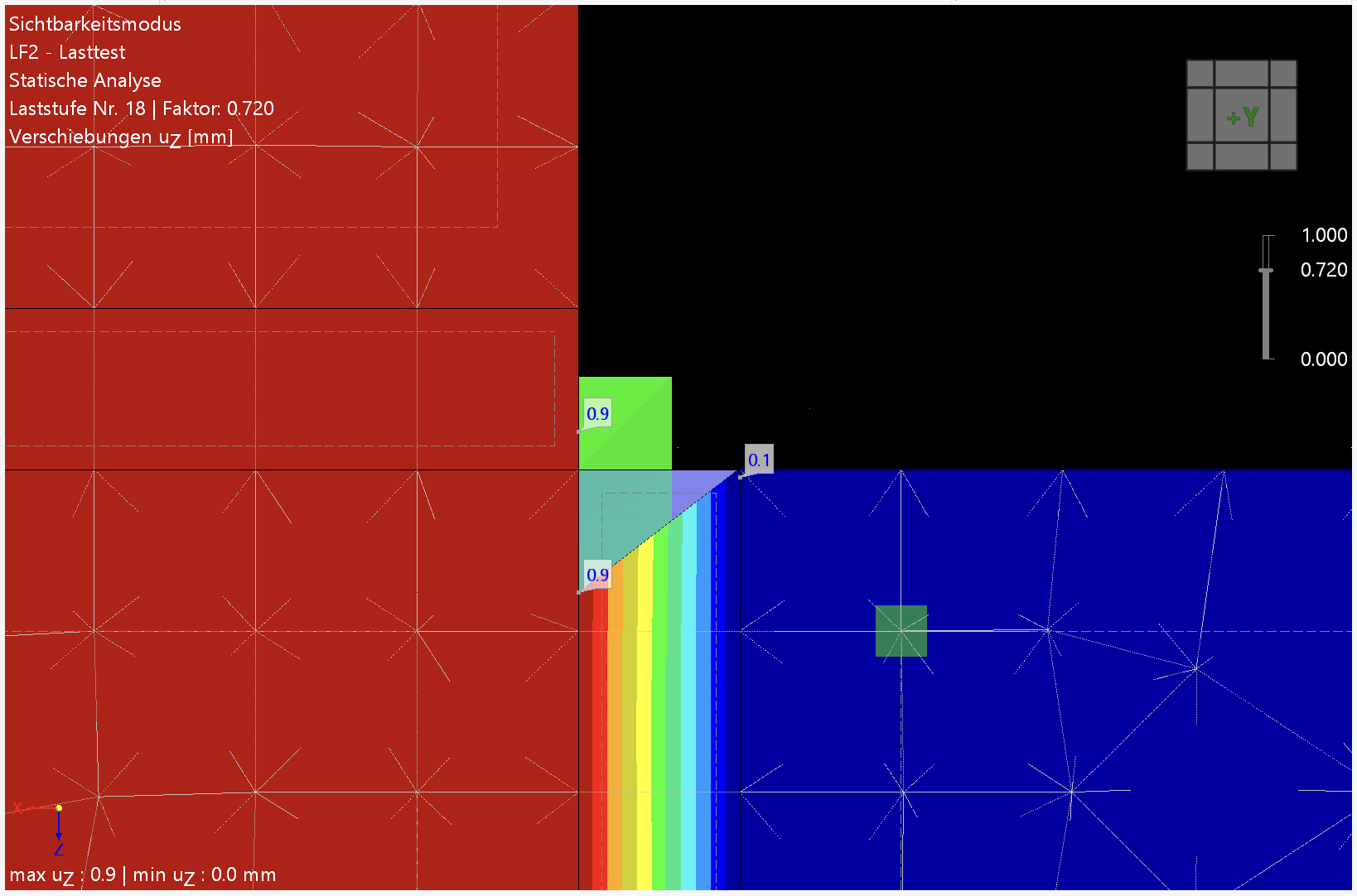
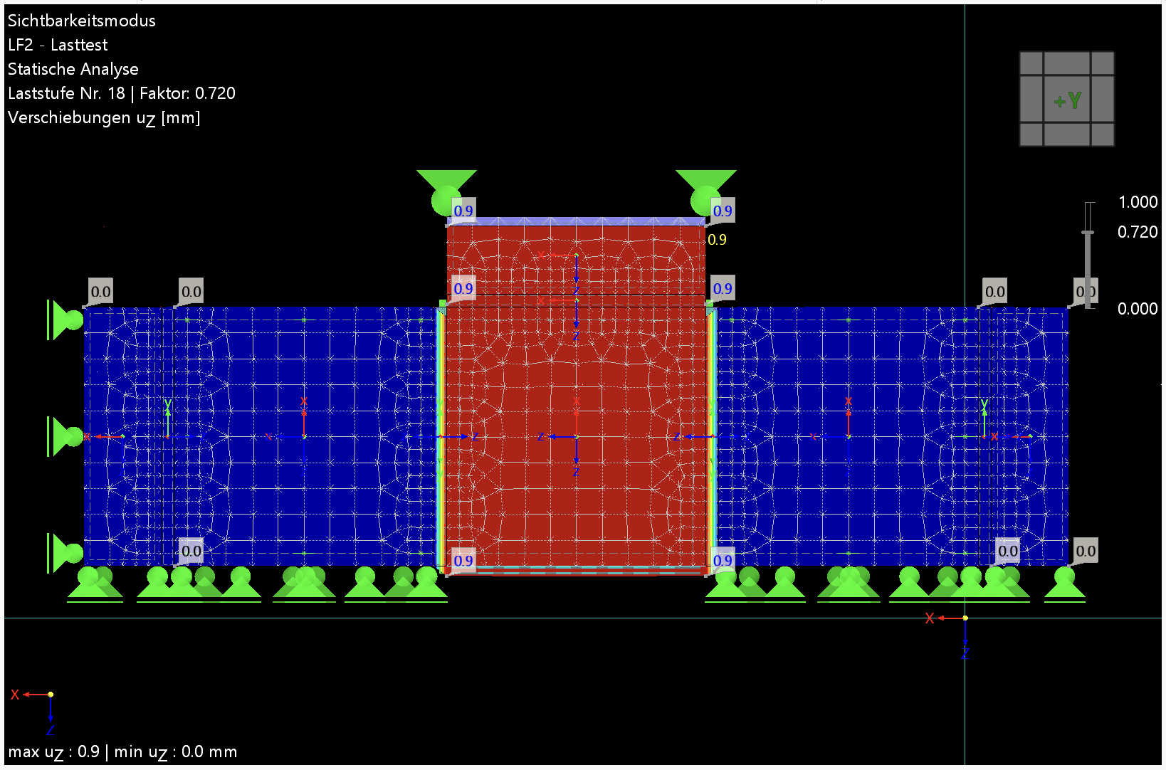
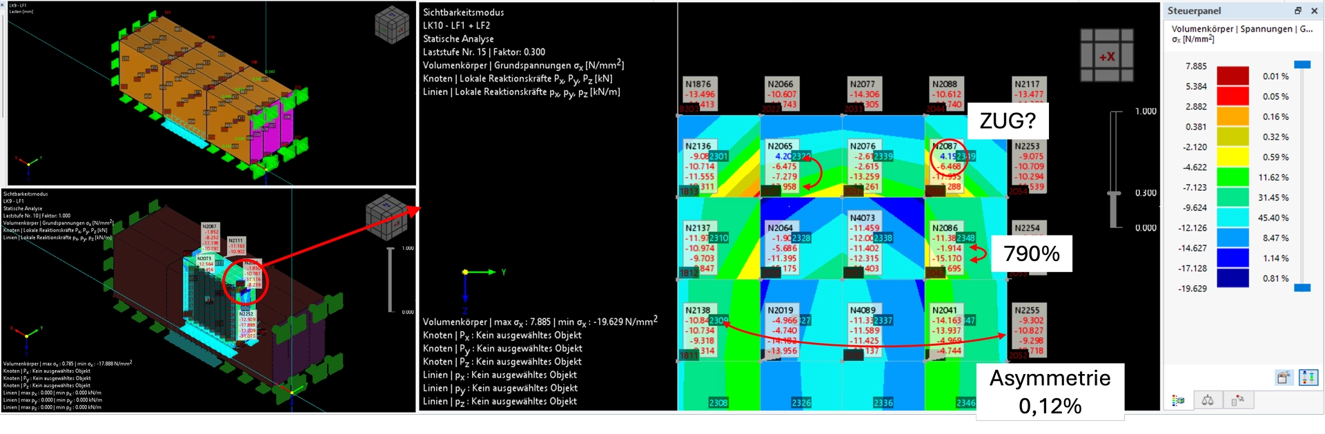
Durch Anpassung der Lasteinleitung im LF1 konnte ich um die X-Z-Ebene beinahe symmetrische Ergebnisse erhalten. Die Abweichungen betragen ca. 0,15%. Ich möchte nachfragen, wie ein in Geometrie und Belastung symmetrisches System zu unsymmetrischen Ergebnissen frühen kann?! Die Asymmetrie tritt sowohl bei der starren Lasteinleitungsfläche der Scherkraft als auch ohne dieser auf.

Reibversuche-Volumenmodell-V31-Holz-Dlubal.rf6 (1,9 MB)

Wenn ich nun bspw. die Spannungen in x-Richtung sigma_x für jeden FE-Knoten anzeige, erhalte ich folgende Ergebnisse. Aufgrund der Dehnsteifigkeiten der Lamellen gehen in die Mittellamelle ca 95% der Vorspannkraft (50kN). Mit einer Fläche von 40mm x 100mm wird eine Spannung von 0,95 x 50000 : (40 x 100) = 11,9N/mm2 erwartet. Die grundsätzliche Größenordnung ist gegeben.
Eine Frage zur grundsätzlichen Auswertung von Ergebnissen an FE-Knoten habe ich in einem Extrabeitrag gestellt (Auswertung FE-Knotenergebnisse). Konkret in diesem Fall sehe ich jedoch teilweise enorme Unterschiede zwischen den einzelnen FE-Knotenergebnissen vor der Glättung.

(zB: N2065: min -17,958N/mm2 bis max +4,20N/mm2)

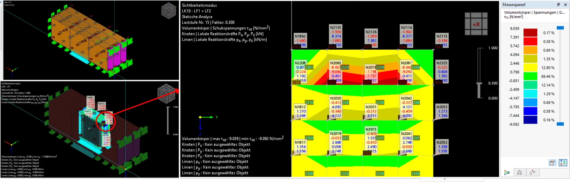
Gegenübergestellt mit den Schubspannungen in dieser Scherfläche tau_xz ergeben sich Werte, die bereits die Haftreibungsgrenze überschreiten und Werte, in denen das nicht der Fall ist. Das bedeutet, dass ein Knoten als Eckpunkt der Fläche A gleitet aber als Eckpunkt der Fläche B noch haftet.
N2065: sigma_x =-17,958;
17,958 x 0,35=6,29 Haftreibgrenze – vorhanden aber tau_xz = -8,6 -> Gleiten
N2065: sigma_x=-6,475;
6,475 x 0,35=2,27 Haftreibgrenze – vorhanden aber tau_xz = 0,457 -> Haften

Im Weiteren beginnt der Körper von oben nach unten nacheinander die Haftgrenze in einzelnen Punkten zu überschreiten. Jedoch sollte die Gesamtlamelle erst zu Gleiten beginnen, wenn in jedem Punkt die Haftgrenze überschritten ist.
Hier beginnt die Gleitung aber, wie weiter oben dargestellt, von Beginn an.
Konkret für Lastfaktor 0,3:
zB:
N2065: sigma_x=-17,958;
17,958 x 0,35=6,29 Haftreibgrenze – vorhanden aber tau_xz= -8,6 -> Gleiten
N2019: sigma_x=-14,183;
14,183 x 0,35=4,964 Haftreibgrenze – vorhanden aber tau_xz= 2,748 -> Haften

Wie geht der solver mit dieser Herausforderung um?
Könnte das der Grund für die zu früh einsetzenden Gleitverschiebungen u_z sein?

Beste Grüße
Alexander