DDES Simulations, Courant Number and y+ Convergence

Hello,

Currently doing an internship on the design of paracyclonic structures, I am using R-WIND 3 to perform advanced aerodynamic analyses. I would need clarifications on the following points:

  1. Averaging of DDES results: In the context of an unsteady flow simulation (DDES), is it possible to perform time averaging of the results (pressure, velocity) directly within the software for data exploitation? If yes, what is the procedure to export or visualize these averaged results?
  2. Display of the Courant number (CFL): To ensure the stability of my unsteady calculations, I would like to monitor the Courant number. Is there an option or a result layer that allows displaying the distribution of the CFL number over the domain?
  3. Issue of y+ and mesh refinement: I am having difficulties reducing the value of y+. Despite local mesh refinement at the structure interface, the value remains too high to properly capture the boundary layer.
  • Does the software limit the thickness of the first boundary layer cell?
  • Do you have any recommendations on the parameters in the "Boundary Layers" tab to enforce a finer wall resolution?

Hello tortuerenard89,
Thank you very much for your questions,

  1. Yes, it is possible to access average values in RWIND when using DDES. I recommend first defining evaluation zones. Then, you can extract the values either via the "Edit Zone Data" option or by using line charts, as illustrated in the figures below:

    image

    image

  2. To monitor the number of Currents, you can check the log file, especially in the RWIND solver transient output section, as shown in the corresponding image:

image

  1. Regarding boundary layer modeling, RWIND currently uses a standard wall function with high y+ values. Unfortunately, it is almost impossible to reach an acceptable y+ range in this setup. I have described the current approach as well as its advantages and limitations in the following knowledge base article, which I recommend you consult:

:backhand_index_pointing_right: https://www.dlubal.com/en/support-and-learning/support/knowledge-base/002040

Please feel free to contact me if you have any further questions,

Best regards,
Mahyar

Thank you very much for your feedback!

1 Like

Hello mahyar.kazemian,

I have a follow-up question regarding access to the Log.file data. It seems that my interface is different from yours: I cannot find this tab when running a DDES (transient) simulation, even though it appears correctly for steady-state studies.

Furthermore, the "Log file" is also inaccessible within the simulation window during the computation.

Could you please help me fix this? For context, I am using RWIND 3 Pro with a student license; does this license type affect the visibility of these features in transient mode?

Thank you in advance for your assistance.

Hello @tortuerenard89,
Thanks for your feedback,

There is also an alternative way to access the log file data. If you can access the temporary file directory, for example, on my system, it is located at (it depends also on your project name):

C:\Users\Public\Documents\Dlubal\RWIND 3.08\Temp~RWIND_Simulation\TBC norm\RF_Simul\Sim001_V01\ofcase0),

Then you will find a file named RWindSolverTransient. This file contains the relevant information:

Please give it a try and let me know if you encounter any issues.

Kind regards,
Mahyar

Hello mahhyar.kazemian,

thank you again for your support !!

i’m still trying to validate some of my CFD results :

In my simulation, I set a convergence criterion for the pressure residual (p) equal to 0.001. However, I would like to better understand the meaning of the residuals F, Fx, Fy, and Fz shown in the residual graph.

According to the RWIND 3 online manual, the residual graph is extended with additional quantities, namely:

  • The force residuals Fx, Fy, and Fz acting on the primary model,

  • The velocity residuals Vx, Vy, and Vz.

My understanding is that the aerodynamic force is obtained by integrating the pressure and shear stresses over the surface of the model. Therefore, since pressure is directly related to the force, I expected the residuals of p and F to show similar convergence trends.

However, in my simulation, the pressure residual and the force residuals exhibit significantly different behaviors.

Could you please clarify the following points?

  1. What exactly does the residual F represent?

  2. Is F the residual of the magnitude of the total aerodynamic force vector?

  3. How are Fx, Fy, and Fz residuals computed?

  4. Why can the force residuals converge differently from the pressure residual, even though the force is derived from the pressure field?

  5. For engineering purposes, should the convergence of F (or Fx) be considered more important than the convergence of p?

Thank you very much for your assistance.

Best regards,

Thibaut Nghiem

Hello Thibaut,

Thank you for the very good and technically relevant questions,

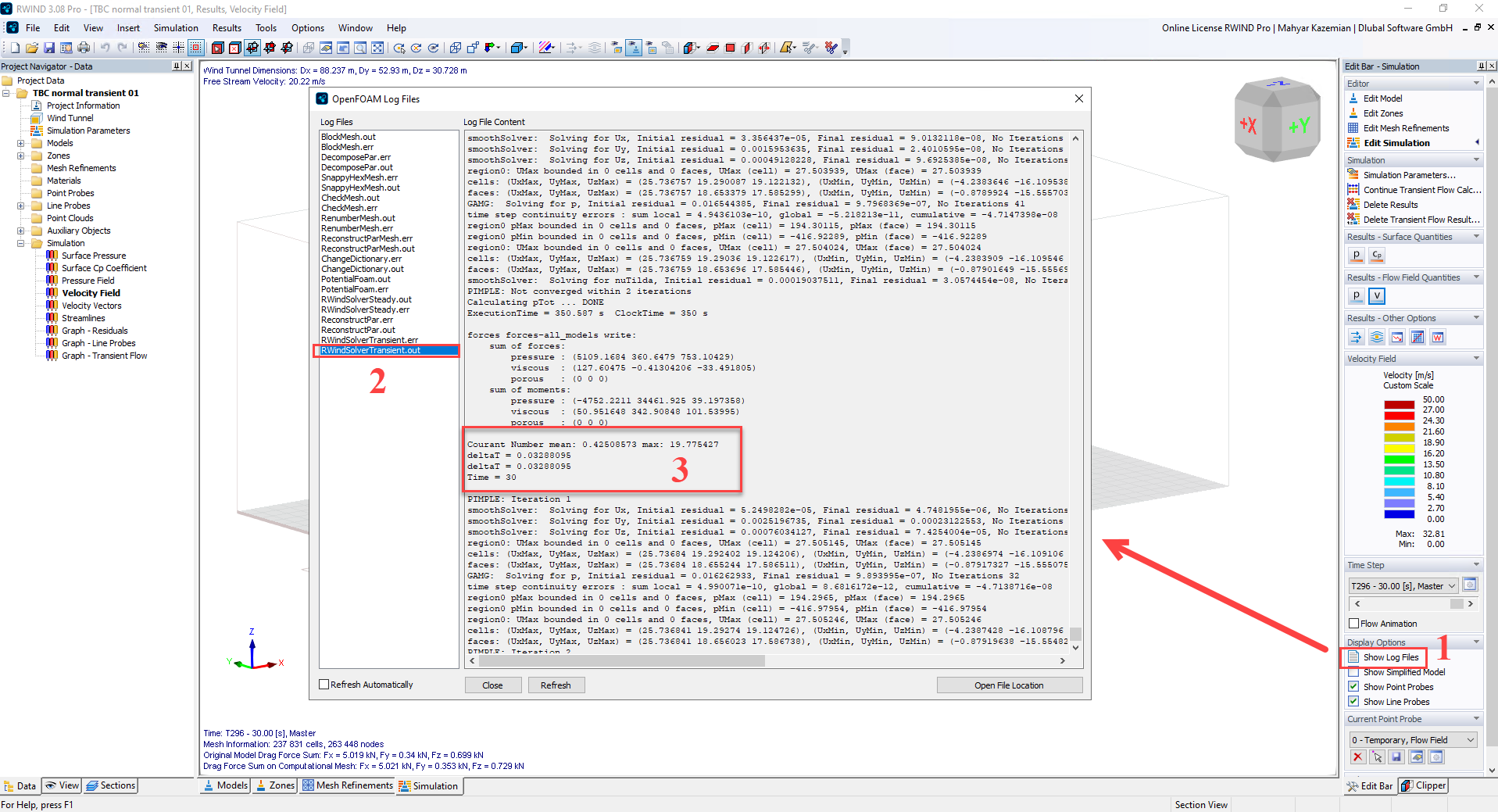
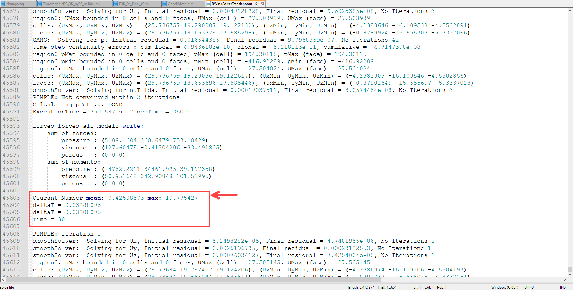
Your interpretation is generally correct: the aerodynamic forces are indeed obtained from the pressure and wall shear stress distributions integrated over the model surface. However, the residuals shown in CFD solvers (including RWIND/OpenFOAM-based workflows) do not necessarily represent the same mathematical quantity, which is why their convergence behavior can differ significantly.

Here is a more detailed explanation.


1. What does the residual F represent?

In RWIND, the quantities:

  • Fx, Fy, Fz

  • and the combined quantity F

are not primary equation residuals like the pressure residual p.

They are instead monitoring quantities derived from the flow solution during the iterations.

In practice:

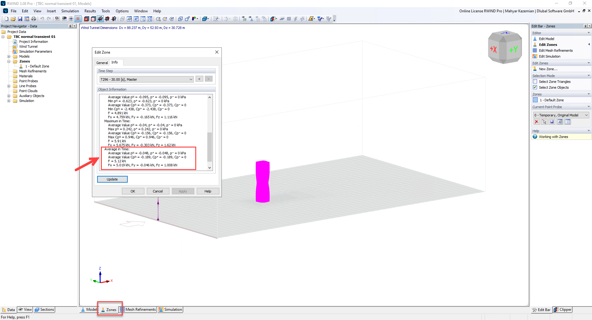
  • Fx, Fy, Fz represent the evolution of the integrated aerodynamic forces acting on the model in each Cartesian direction.

  • F is typically the resultant (magnitude) of the aerodynamic force vector:

image

So the plotted “force residuals” are usually related to the iteration-to-iteration variation of these integrated forces rather than the algebraic residual of a discretized transport equation. This is an important distinction.


2. How are Fx, Fy, and Fz computed?

The aerodynamic forces are computed by integrating:

  • pressure forces (normal stresses),

  • and viscous/shear forces (tangential stresses)

over the model surface.

In continuous form:

where:

  • p = pressure,

  • n = surface normal vector,

  • tau = viscous shear stress tensor.

The directional components are then:

Numerically, RWIND/OpenFOAM evaluates these quantities after every iteration from the current flow field solution.


3. Why can force residuals behave very differently from pressure residuals?

This is actually very common in CFD. The key reason is that:

The pressure residual measures the local algebraic convergence of the pressure equation, while force monitors are global integral quantities.

These are fundamentally different metrics.

Pressure residual (p)

The pressure residual represents how well the discretized pressure equation is satisfied between successive iterations.

It is sensitive to:

  • local cell imbalance,

  • mesh quality,

  • pressure correction steps,

  • under-relaxation,

  • local recirculation regions.

It is therefore a field equation convergence metric.


Force monitors (Fx, Fy, Fz)

The forces are surface-integrated quantities.

Because of the integration:

  • local pressure oscillations may cancel out,

  • errors in different regions may compensate each other,

  • small local non-converged regions may have negligible effect on total force.

Therefore, it is completely possible that:

  • pressure residuals still fluctuate,

  • while aerodynamic forces are already nearly stable.

The opposite can also happen:

  • pressure residuals appear low,

  • but forces still oscillate due to vortex shedding, separation instability, or insufficient physical convergence.


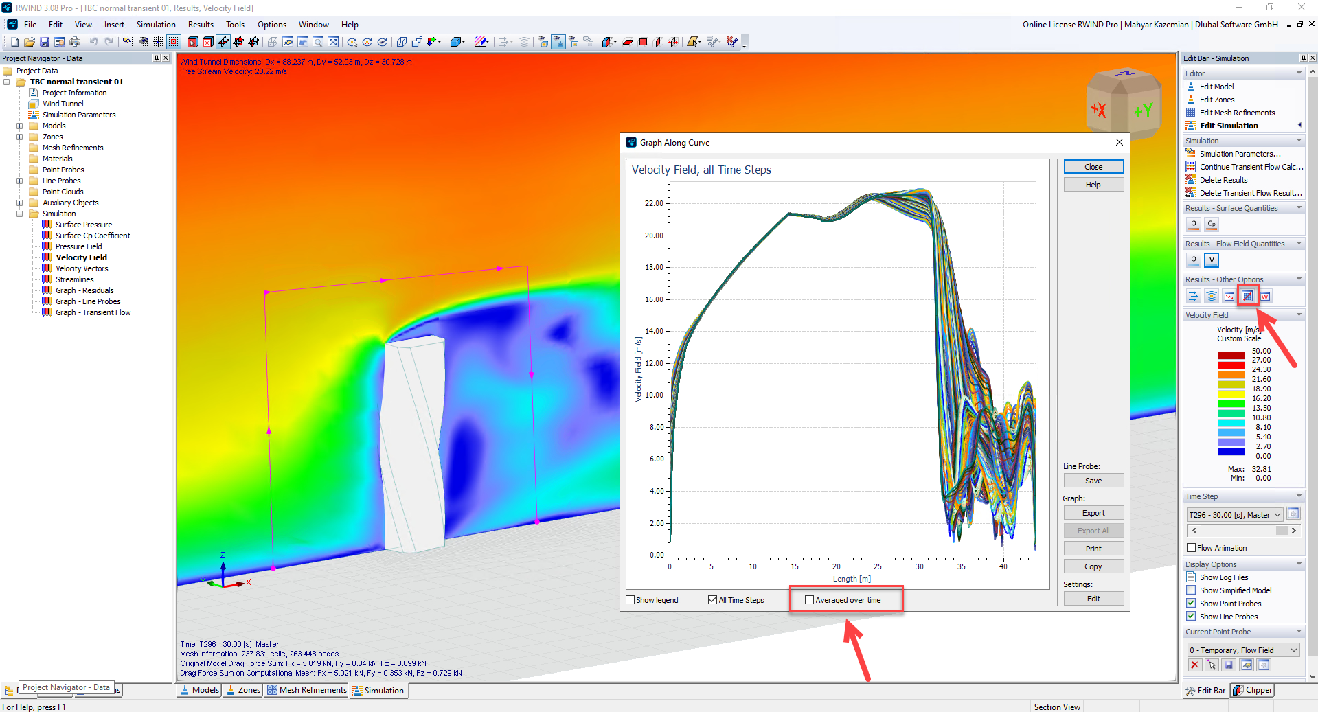
4. Why are your force residuals oscillating?

From your graph, the behavior suggests:

  • The pressure residual decreases relatively smoothly,

  • while especially one force component (likely Fy) shows strong oscillations.

This usually indicates one of the following:

A) Physical unsteadiness in the flow

For separated bluff-body flows:

  • vortex shedding,

  • wake instability,

  • shear layer oscillation

can produce fluctuating integrated forces even in nominally “steady” RANS calculations.

This is very common around:

  • sharp corners,

  • roof edges,

  • cylinders,

  • curved roofs,

  • membrane structures.


B) Sensitivity of integrated forces

The total force may be highly sensitive to:

  • separation point movement,

  • local recirculation zones,

  • wake asymmetry.

A tiny change in separation can strongly modify integrated lift/side force while pressure residuals remain relatively small.


C) Numerical reasons

Force monitors are also more sensitive to:

  • mesh refinement near separation zones,

  • wall treatment,

  • y+ distribution,

  • turbulence model behavior,

  • relaxation factors.


5. Should force convergence be considered more important than pressure convergence?

For engineering CFD, usually:

The convergence of engineering target quantities is more important than residuals alone.

So if your objective is:

  • global wind loads,

  • drag coefficients,

  • base reactions,

  • structural loading,

then stabilization of:

  • Fx,

  • Fy,

  • Fz,

  • Cp averages,

is often more important than achieving an extremely low pressure residual.


However, this does not mean residuals are irrelevant.

A good engineering CFD solution normally requires BOTH:

Numerical convergence

Residuals sufficiently reduced.

Typical practical ranges for steady RANS:

  • (10^{-3}) → acceptable engineering level,

  • (10^{-4}) or lower → preferable,

  • Lower may be needed for sensitive flows.


Physical convergence

Monitored quantities become statistically stable:

  • forces,

  • moments,

  • pressure coefficients,

  • velocity probes.


6. Which criterion is usually more meaningful in practice?

For wind engineering applications:

Quantity Importance
Pressure residual Numerical convergence indicator
Velocity residuals Flow-field stabilization
Fx/Fy/Fz stabilization Engineering load convergence
Cp stabilization Local pressure reliability

For structural wind engineering, many engineers actually trust:

  • stable force coefficients,

  • stable Cp distributions,

  • and mesh-independence studies

more than residual values alone.


7. Important practical remark for RWIND / steady RANS

For strongly separated aerodynamic flows, a perfectly monotonic residual decay is often unrealistic. Especially for:

  • sharp-edged buildings,

  • canopies,

  • tensile membranes,

  • free-form roofs,

  • stadiums,

small oscillations in force monitors are expected.

Therefore, the key question is usually:

Are the monitored engineering quantities fluctuating around a statistically stable mean?

rather than:

Did every residual reach an arbitrarily low value?


8. Recommended validation workflow

For engineering validation, I would recommend:

Step 1 — Residual monitoring

Ensure residuals decrease sufficiently:

  • preferably below (10^{-3}),

  • ideally toward (10^{-4}).


Step 2 — Monitor forces

Check whether:

  • Fx,

  • Fy,

  • Fz

reach stable mean values.


Step 3 — Mesh sensitivity study

Compare:

  • global forces,

  • Cp distributions,

  • separation regions

across multiple meshes.

This is often more important than residual magnitude alone.


Step 4 — Compare with references

If possible:

  • wind tunnel data,

  • Eurocode expectations,

  • literature benchmarks,

  • AIJ/ASCE validation cases.


Please let me know if you have more questions,

Best regards,
Mahyar Kazemian

3 Likes